Procedural Whodunnits #1, Motives and Means

There’s a strong argument from Jimmy Maher that the whodunnit lends itself uniquely well to game design, in that no other literary genre sees itself so explicitly “as a form of game between reader and writer”. There’s an equally strong argument that trying to procedurally generate whodunnits is a doomed and deeply stupid venture. For a design problem with such a rich history of misfires and mistakes, from Sheldon Klein’s mystery generator (1973) to Murder of the Zinderneuf, you’ve got to ask - why do this?

I am a sucker for murder mysteries. Five Little Pigs unfailing makes me misty-eyed, Knives Out is a yearly rewatch, and I ardently believe Return of the Obra Dinn is one of the best things to ever happen to the genre. Between that and the Golden Idol series, the design space for deductive games has undoubtedly opened up in recent years, but I find both lack the simple human drama of gathering a bunch of characters in a room and letting them talk. I wanted to make a more dialogue-driven puzzle centred around that moment of the whodunnit… and not just because it’s easier to write a bunch of text than it is other assets.

The other problem baked into these stories is, well, you can only really experience them once. Yes, yes, it’s all good fun to reread/rewatch/replay a mystery and see all the clues hidden in plain sight, but it’s not the same now is it? Just look at the reviews for Obra Dinn: you can hardly move for players wishing they could experience it for the first time again. To me, the whodunnit represents a holy grail for procedural storytelling: where players (self included) can experience similar, but not the same, puzzles as many times as they wish¹. They have the space to learn how the generator works, and can easily look up details about it online, without having any solutions spoiled per se.

^{1Well, at least until perceptual collapse sets in. I highly recommend Generator's Haunted by Max Kreminski for an explaination of the phenomenon, where they describe the experience of building a mental model of the generator from its output. I'll be the first to admit that any generator will only ever produce so much variety... but that won't keep me from using the phrase "infinitely replayable" all the same.}

All of this is to say, I’ve got a lot to write about here. In this - sporadic - series of blogs, I’m going to talk through the core features of my generator and the thinking behind them, the how and the why as it were. Some posts will be inevitably more design-focused, some more technical (it’s unlikely there’ll be any on the art direction, I doubt I’ll have all that much to contribute in that area). I’ll be writing them as much as to help myself keep track of what hasn’t worked as let other devs know what has. So, without further ado…

Representation

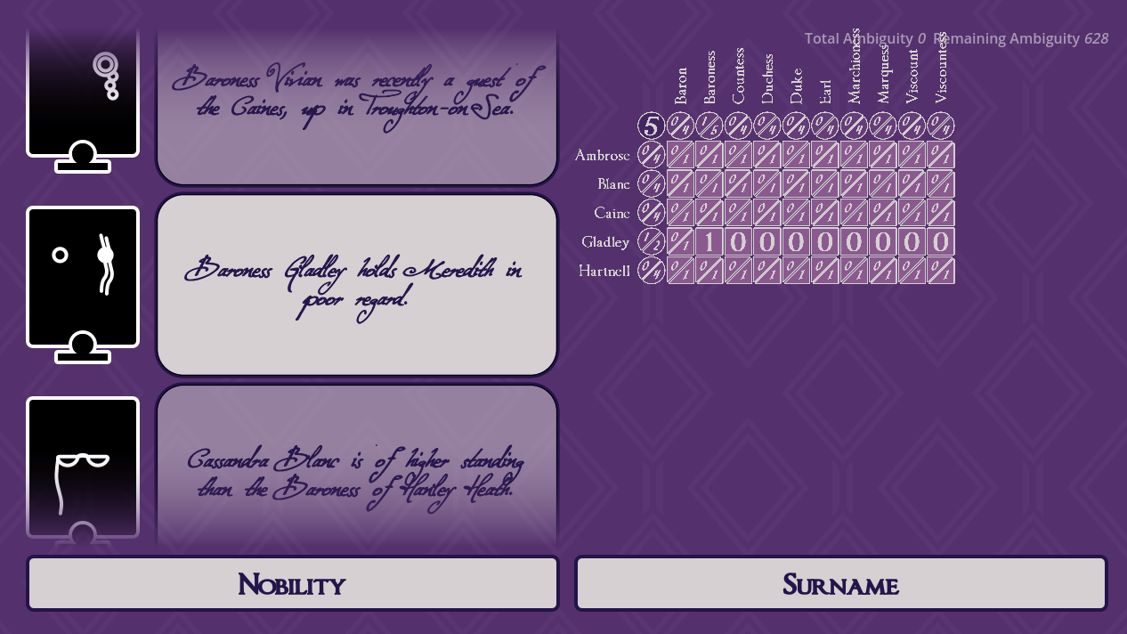
At its lowest level, Bad Bohemians is an exercise in generating logic puzzles - specifically, Einstein puzzles. Given \(n\) forenames, \(n\) surnames, etc., the player is tasked each element from each category to one of \(n\) different characters. The player can do this by filling up a grid with ticks and crosses; in code, they’ll be replaced with closed intervals \([\min,\max]\).

The idea here is, we need a way of representing our puzzles and their possible solutions in a form the computer can understand. This is not a natural language processing project; the computer won’t get any information out of even a clue like Character #1 is called Abigail as written. However, if we tag that clue with constraint \((1, \textrm{Abigail}) \in [1,1],\) the code has a solver that will read this and tighten the bounds at its \((1, \textrm{Abigail})\) coordinate to a minimum of $1$, and a maximum of… well, in this case, also \(1.\)

We won’t concern ourselves with where those constraints are being written just yet, that’s a problem for our text generator. What matters here and now is we’ve got a tried-and-tested data structure that our solver can read information into to then make deductions from. That said, this grid, while perfectly suitable for pen-and-paper Einstein puzzles, actually encodes several assumptions about which solutions may or may not be valid. In order to generate a broader and more narratively interesting range of whodunnits, we’re going to need to extend our model to remove some of those limitations.

Generalisation

Here’s what I mean. Right now, we’re assuming each element is used exactly once, which eliminates the possibility of mistaken identities, where, e.g., two characters share the same forename. This assumption is restricting narrative possibilities; the above model needs generalised. By assigning bounds to not only 2D coordinates of \(\{\textrm{forename}, \textrm{surname}\}\) square, but also the 1D coordinates along our \(\{\textrm{forename}\}\) and \(\{\textrm{surname}\}\) lines, we can surely enough bake in the possibility of forenames and surnames appearing more than once. While we’re at it, we’ll also go ahead and assign a bound to represent the total number of characters in the puzzle.

As a collorary to the above, these 1D bounds can also introduce red herrings. Bad Bohemians’ characters, for instance, are members of the landed gentry, and so each has an associated \(\{\textrm{nobility}\}\). The British aristocracy has five ranks of peerage, from Dukes and Duchesses down to Barons and Baronesses, so a total of 10 possible titles. We can comfortably include a category like this, with more elements than our puzzle has characters, because our model now allows for elements that aren’t used even once!

Another scenario, suppose we received the clue Character #1 is either called Adeline, or is a Byron. A player might read that and decide to come back to it once they’ve eliminated either Adeline or Byron as an option, but what about the computer? Just as we’ve added 1D bounds to our model, we can as well extend it in the other direction with a 3D \(\{\textrm{character}, \textrm{forename}, \textrm{surname}\}\) grid. Rather than waiting to use the clue, the solver immediately bounds coordinate \((1,\textrm{Abigail}, \textrm{Byron})\) and all of set

\[\{(1,\textrm{forename}, \textrm{surname}):\textrm{forename}\neq\textrm{Abigail},\textrm{surname}\neq\textrm{Byron}\}\]

to zero. Indeed, we can generally create any \(D\)-dimensional grid to contain the information about \(D\) related categories!

Deductions

Here, it becomes helpful to organise these different dimensions of grid into a single hierarchy. For a puzzle with \(D\) categories total, at the top of this hierarchy is that single bound for the total number of characters we mentioned earlier, which can be thought of as a 0-dimensional point. Below that are all \(D\) of the puzzle’s 1-dimensional rows, below those all \(\frac{1}{2}D(D-1)\) of its 2-dimensional squares, and so on. Combinatorics enjoyers will note this hierarchy has exactly \(D\) choose \(d\) grids of dimension \(d\), all the way down to a single, \(D\)-dimensional entry over all possible categories. It encodes every possible detail of every possible character, meaning a puzzle will be solved if and only if each of this grid’s bounds is tightened to a single value. We will therefore call it our primary grid.

Next, the \(2^D\) grids are connected up: for each layer \(1 \leq d \leq D\), we go through and bind each grid to the \(d\) grids in the layer above containing some subset of its categories. We could describe these connections as forming the \(D\)-dimensional hypercube graph \(Q_D\), if we were being particularly rigourous about it.

It took a bit of setup, but this is the data structure our solver relies on to make its deductions. As discussed, the solver will register information by tightening the bounds of the relevant grid - but what I’ve conspicuously missed out until now is it also propagation that information upwards and downwards to the grids adjacent. This is how the solver, just like the player, makes deductions: taking elementary facts about the higher levels of the hierarchy (say, that Character #1 is called Abigail) and piecing them together to resolve the primary grid.

How does this information trickle down, though? Whatever algorithm we use, it’ll need to work over any number of \(d\) dimensions, for any grid \(\mathbf{E} = \{E_1, ..., E_d\}\) made up of categories \(E_i\). We’ll start with that general case, but don’t worry - I’ll include some much more tangible examples further on.

Let’s start with the obvious. If \(\mathbf{E}\) has a coordinate

\[\mathbf{e} = (e_1, ..., e_d) \in [e_{\min}, e_{\max}],\]

then any grid \(\mathbf{F} = \{\mathbf{E}, F\} = \{E_1, ..., E_d, F\}\) directly below it must have all coordinates

\[\mathbf{f} = (\mathbf{e}, f) = (e_1, ..., e_d, f) \in [0, e_{\max}]\]

…which isn’t actually all that much to go on. It’ll be much more instructive to consider the row of coordinates \(\mathbf{F}_{\mathbf{e}} = \{(e_1, ..., e_d, f): f \in F\}\) all at once. Denoting the bounds of each \(\mathbf{f}\) as \([f_{\min}, f_{\max}]\), they must satisfy

\[e_{\min} \leq \sum_{f \in F} f_{\max}, \;\; e_{\max} \geq \sum_{f \in F} f_{\min}.\]

As such, when any bound of any \(\mathbf{f}\) is tightened, our solver algorithm will propagate that information upwards to all grids \(\mathbf{E}\) by mapping

\[e_{\min} \mapsto \max\left(e_{\min}, \, \sum_{f \in F} f_{\max}\right), \;\; e_{\max} \mapsto \min\left(e_{\max}, \, \sum_{f \in F} f_{\min}\right)\]

as appropriate.

Bounding \(\mathbf{f}\) can just as well fire information across \(\mathbf{F}\). For any other \(\mathbf{f}'\) in the same row \(\mathbf{F}_{\mathbf{e}}\), we can rearrange the above inequalities as

\[f_{\max}' \geq e_{\min} - \sum_{f \neq f'} f_{\max}, \;\; f_{\min}' \leq e_{\max} - \sum_{f \neq f'} f_{\min}.\]

This does not seem terribly useful in itself (we need an lower bound on \(f_{\min}'\) after all), but take a step back. We’re tightening the minimum and maximum of \(f'\) until they converge on a single value, so if we know \(f_{\min}'\) is bounded above we can safely lower \(f_{\max}'\) to that upper bound, and vice versa! Therefore, the algorithm will also map

\[f_{\min}' \mapsto \max\left(f_{\min}', \, e_{\min} - \sum_{f \neq f'} f_{\max}\right), \;\; f_{\max}' \mapsto \min\left(f_{\max}', \, e_{\max} - \sum_{f \neq f'} f_{\min}\right)\]

(a mapping that propagates information not only across, but also downwards from \(\mathbf{E}\) to \(\mathbf{F}\) as \(\mathbf{e}\) tightens).

Limitations

Right then, that seems like as good a place to pause as any. We’ve seen how Bad Bohemians will model its puzzles using an underlying grid structure, how these grids have been generalised to allow a wider variety of clues, and how they connect up, so that regardless of where new information is injected into the solver, it can propagate out in all directions. I’ve kept the explainer abstract and mathematical so far because, well, the model is still an abstraction. This post sets out how the solver will ideally work, but those ideals are about to crash up against the harsh realities of code: as the CPU goes about manipulating this massive data structure, we’ll have to work around some of these with clever/not-so-clever optimisations, others by adapting our design. See you then.